Using Machine Learning To Tease Out A Dynamic Pricing Algorithm
On November 29, 2013, I wrote a piece titled “Not Worth the Cost: A 17-Month Case Study of Congestion Pricing in the SF Bay Area.” In that piece, I presented data I manually collected on toll costs for the westbound Express Lane on Highway 237 (running from Milpitas to Sunnyvale, CA) versus the drive time on the highway’s general purpose lanes. I was disappointed to find that the relationship between the two was not very reliable. Moreover, I concluded that neither the toll nor the overall projects costs are worth paying.
Motivated by comments and questions from a reader, I decided to take a deeper look at the data to see whether I could tease out some more complex relationships. I will be doing this analysis in stages. In this first stage, I developed a simple machine learning model using a regression tree to predict drive times based on a full array of variables.
I broke up the data into the following independent variables:
- Cost: price of the toll on the Express Lane in dollars.
- Month: index for month of the year (1=Jan, 2=Feb, etc…) using the date of the data collection.
- DayofWeek: index for the day of the week (2=Mon, 3=Tue, etc..) using the date of the data collection. Note that the tolls only apply on non-holiday weekdays.
- WeekOfYear: index for the week of the year (1=the first week which is Jan 1st, 2 = the second week, etc..) using the date of the data collection. Note that the week starts on Monday.
- Hour: the hour component of the start time of the drive on the general purpose lane.
- Minute: the minute component of the start time of the drive on the general purpose lane.
The dependent variable (what the model is trying to predict/classify) is the duration of the drive on the general purpose lane in seconds. I coded this as DriveTimeSeconds.
I used the e1071 package in R for creating the best regression tree using 10-fold cross-validation.
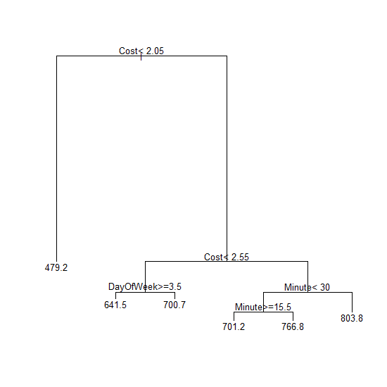
The initial results are promising. The regression tree below shows that drive time on the general purpose lane is influenced by the day of the week and the fraction of the hour (but NOT the hour itself!). Adding these variables to the cost information from the toll lanes provides a richer understanding of resulting drive times. Of course, the model cannot know whether congestion itself depends on the day of the week and the time, but, for now, congestion does not appear to be material to this model since I generally did not observe congestion in the Express Lane during my data collection. Ironically, the last two days that I added to the data – December 3rd and 6th – DO include some observed (very minor) congestion in the Express Lane.

Here is how to interpret the branches of the tree (from left to right of the leaf or end nodes):
- If the cost of the Express Lane is less than $2.05, then I can an average drive time of 479.2 seconds (8.0 minutes).
- If the cost is less than $2.55 but at least $2.05 AND the weekday is a Wednesday, Thursday, or Friday, then I can expect an average drive time of 641.5 seconds (10.7 minutes).
- If the cost is less than $2.55 but at least $2.05 AND the weekday is a Monday or Tuesday, then I can expect an average drive time of 700.7 seconds (11.7 minutes).
- If the cost is at least $2.55 AND the time is before half past the hour AND the time is at least 15.5 minutes past the hour, then I can expect an average drive time of 701.2 seconds (11.7 minutes).
- If the cost is at least $2.55 AND the time is before 15.5 minutes past the hour, then I can expect an average drive time of 766.8 seconds (12.8 minutes).
- If the cost is at least $2.55 AND the time at least 30 minutes past the hour, then I can expect an average drive time of 803 seconds (13.4 minutes).
With these results, I can move beyond the disappointing scatter of the 2-dimensional graph of drive time versus cost and see the more complex relationships at work. It is VERY interesting to see that while the tolls ranged from $0.85 to $4.25, the tree only contains two branching points based on cost. This verifies that cost is not a sufficient determinant of average driving time from the perspective of the driver in the general purpose lane.
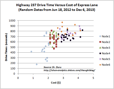
The chart below recasts the original chart: it color-codes the points according to the rules from the regression tree. You can now visualize how the algorithm partitioned the data. The “nodes” in the legend are ordered and numbered as shown in the list above.

(Random Dates from Jun 18, 2012 to Dec 6, 2013)
With this format, you can also visualize which parts of the model have the highest error rates. The very first rule, “Node1”, has the highest error rate given that with a cost less than $2.05 drive time can range from 200 to 800 seconds (3.3 to 13.3 minutes). If I had additional variables at my disposable, I might be able to reduce the error rate of this region of data. This model can also be a starting point to help the VTA generate a more consistent congestion pricing model (again, from the perspective of the general purpose driver).
In a future analyze, I will apply k-means clustering to these data to see whether I can generate even richer results. I think the partitioning routine of k-means should be well-suited to this problem. I will also explore metrics of performance of these models. Stay tuned!
(Author’s addendum for December 7, 2013: I neglected to include a variable for the year in the above analysis. Such a variable is very effective in detecting whether the VTA’s pricing algorithm has experienced significant change over time. After adding in the year, the model did not change. However, going forward, I will keep this variable so that any significant changes do get flagged.)

Hey Duru! I’m loving these analyses a lot! I see what you did. Creating a decision tree for commute times and color coding the nodes on the same plot from last time is way better than arbitrarily assigning low/med/high categories. A few questions and comments: 1) Is it possible to use other variables to break the decision tree, like weather or a binary variable for accident/no accident? Or I guess, would you want to?
2) Instead of using the current minute and hour variable, would it be better to use a minute variable that contains values from 0 (12am) – 1440 to denote the time of day?
3) Can’t wait for the k-means on this data. Based on your updated graph, I’m seeing 3 clusters, first for node 1, second for node 2-3 and third for node 4-6. Can that represent different tiers of traffic conditions?
4) Based on your results, I’m trying to interpret the meaning of a high error present for nodes 1-3. For example, if they price it <= $2.05, there's a wide range of commute times for general purpose, meaning it's a toss up for how many people actually use the express lane at that price point? Priced above $2.55, it's not going to affect the commute time in the general purpose lane. But is that because it's too expensive for drivers or because it has no impact on the general use lanes due to the sheer amount of existing traffic?
4) High prices are associated with high commute times in the general use. That's probably normal because high traffic times are when they would increase the price to use the express lane. I'm wondering if there's a way to generate a baseline commute time to understand the true effects of the pricing of express lane. For example, the average commute times for nodes 4-6 or (2-3); how's that compare for the average commute time of those days without the express lane? Of course, there's no way to get that number, but are there any methods for generating a proxy for it?
Thanks so much for doing this analysis, I'm really enjoying it!